相机模型
阅读《Multiple View Geometry in Computer Vision》,摘录部分重点。
Finite cameras
The basic pinhole model
Consider the plane $\mathrm{Z}=f$, which is called the image plane or focal plane.
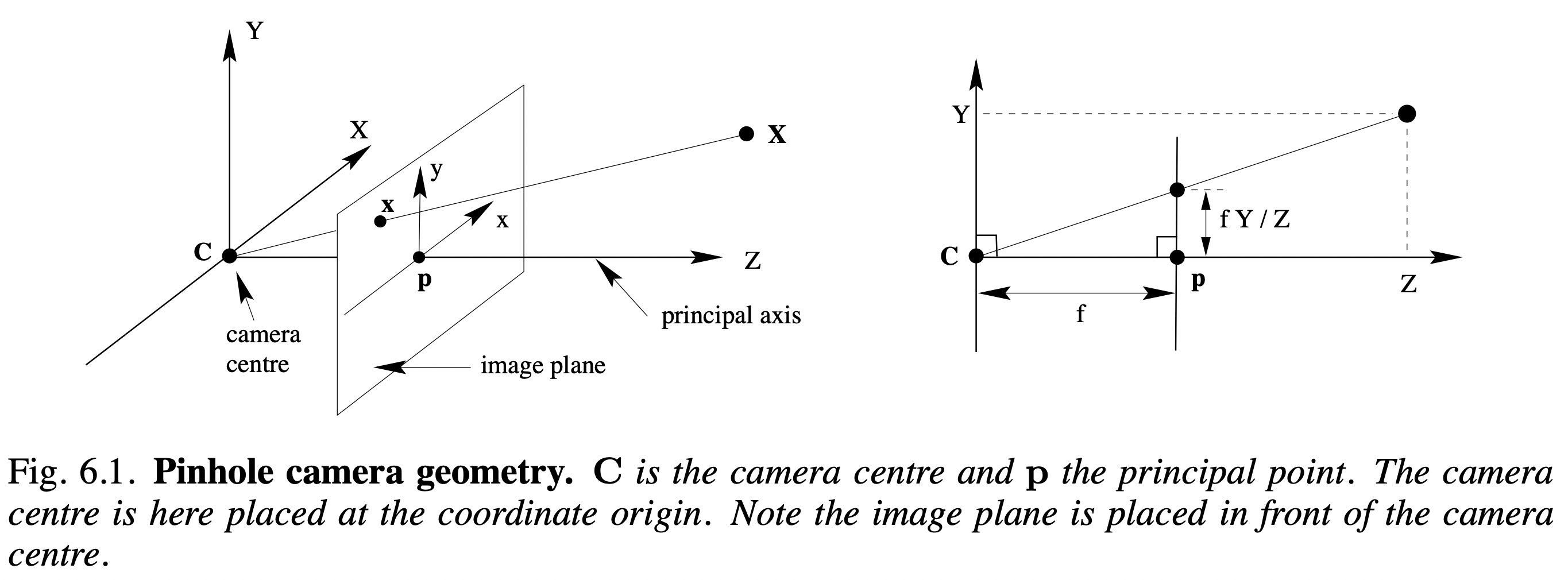
A point in space with coordinates $\mathbf{X}=(\mathrm{X},\mathrm{Y},\mathrm{Z})^{\top}$ is mapped to the point $(f\mathrm{X}/\mathrm{Z},f\mathrm{Y}/\mathrm{Z},f)^{\top}$ on the image plane. Ignoring the final image coordinate, we see that
\[(\mathrm{X},\mathrm{Y},\mathrm{Z})^{\top} \mapsto (f\mathrm{X}/\mathrm{Z},f\mathrm{Y}/\mathrm{Z})^{\top}. \tag{1} \label{eq6-1}\]Central projection using homogeneous coordinates
\[\left(\begin{array}{l} \mathrm{X} \\ \mathrm{Y} \\ \mathrm{Z} \\ 1 \end{array}\right) \mapsto\left(\begin{array}{c} f \mathrm{X} \\ f \mathrm{Y} \\ \mathrm{Z} \end{array}\right)=\left[\begin{array}{llll} f & & & 0 \\ & f & & 0 \\ & & 1 & 0 \end{array}\right]\left(\begin{array}{l} \mathrm{X} \\ \mathrm{Y} \\ \mathrm{Z} \\ 1 \end{array}\right) \tag{2} \label{eq6-2}\] \[\left[\begin{array}{llll} f & & & 0 \\ & f & & 0 \\ & & 1 & 0 \end{array}\right] \implies \operatorname{diag}[f, f, 1](\mathtt{I} \mid \mathbf{0})\]We now introduce the notation
- $\mathbf{X}$ for the world point represented by the homogeneous 4-vector $(\mathrm{X}, \mathrm{Y}, \mathrm{Z}, 1)^{\top}$
- $\mathrm{x}$ for the image point represented by a homogeneous 3-vector
- $\mathtt{P}$ for the $3 \times 4$ homogeneous camera projection matrix.
Then $\eqref{eq6-2}$ is written compactly as
\[\mathbf{x}=\mathtt{P}\mathbf{X}\]which defines the camera matrix for the pinhole model of central projection as
\[\mathtt{P}=\operatorname{diag}[f, f, 1](\mathtt{I} \mid \mathbf{0}).\]Principal point offset
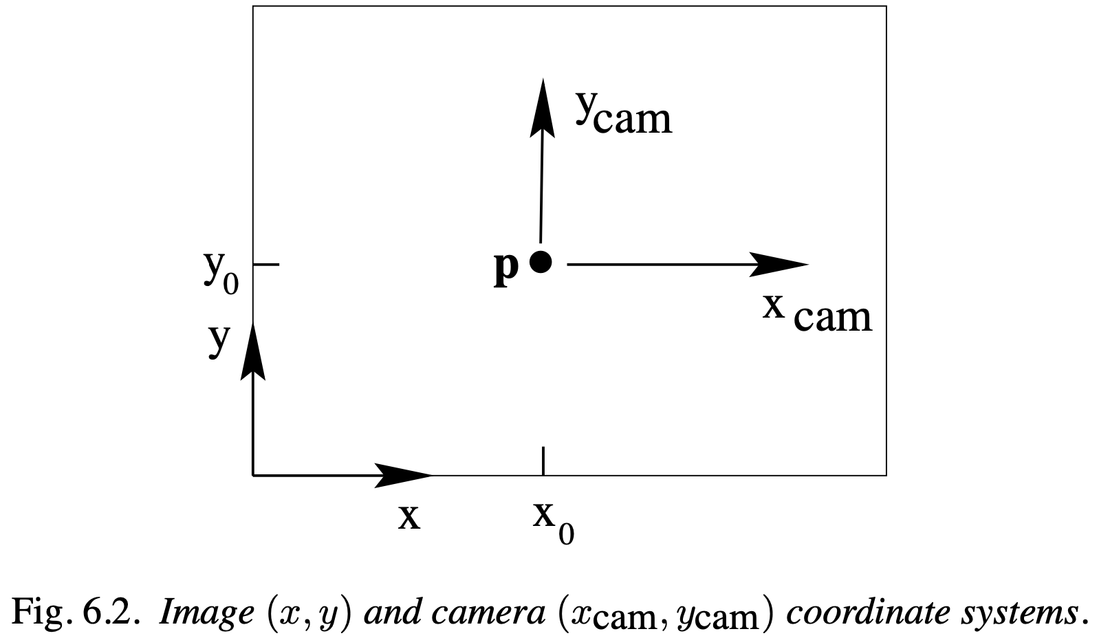
Principal point offset. The expression $\eqref{eq6-1}$ assumed that the origin of coordinates in the image plane is at the principal point. In practice, it may not be, so that in general there is a mapping
\[(\mathrm{X}, \mathrm{Y}, \mathrm{Z})^{\top} \mapsto\left(f \mathrm{X} / \mathrm{Z}+p_{x}, f \mathrm{Y} / \mathrm{Z}+p_{y}\right)^{\top}\]where $\left(p_{x}, p_{y}\right)^{\top}$ are the coordinates of the principal point. See figure 6.2. This equation may be expressed conveniently in homogeneous coordinates as
\[\left(\begin{array}{c} \mathrm{X} \\ \mathrm{Y} \\ \mathrm{Z} \\ 1 \end{array}\right) \mapsto\left(\begin{array}{c} f \mathrm{X}+\mathrm{Z} p_{x} \\ f \mathrm{Y}+\mathrm{Z} p_{y} \\ \mathrm{Z} \end{array}\right)=\left[\begin{array}{cccc} f & & p_{x} & 0 \\ & f & p_{y} & 0 \\ & & 1 & 0 \end{array}\right]\left(\begin{array}{c} \mathrm{X} \\ \mathrm{Y} \\ \mathrm{Z} \\ 1 \end{array}\right) \tag{3} \label{eq6-3}\]Now, writing
\[\mathtt{K}=\left[\begin{array}{ccc} f & & p_{x} \\ & f & p_{y} \\ & & 1 \end{array}\right]\]then $\eqref{eq6-3}$ has the concise form
\[\mathbf{x}=\mathtt{K}[\mathtt{I} \mid \mathbf{0}] \mathbf{X}_{\text {cam }} .\]The matrix $\mathrm{K}$ is called the camera calibration matrix. In (6.5) we have written $(\mathrm{X}, \mathrm{Y}, \mathrm{Z}, 1)^{\top}$ as \(\mathbf{X}_{\text{cam}}\) to emphasize that the camera is assumed to be located at the origin of a Euclidean coordinate system with the principal axis of the camera pointing straight down the Z-axis, and the point \(\mathbf{X}_{\text{cam}}\) is expressed in this coordinate system. Such a coordinate system may be called the camera coordinate frame.